This post explores some of the the data I collected from the IGM Experts Forum, which surveys a group of leading economists on a variety of policy questions. A CSV of all the data is available here, as are separate datasets of the questions and responses. An IPython notebook with all of the code from this analysis is available here.
I’m especially interested in how confidence changes with the scale of a claim, so I use a few different techniques to look at that relationship. First, I look at confidence by vote type and find that economists seem to be more confident when they strongly agree or strongly disagree. Second, I find that confidence actually increases the further a view is from the median, although this is relationship is mainly driven by 25 votes out of a 7024 vote sample.
An earlier paper [1, PDF] by Gordon and Dahl found that male economists and economists that were educated at the University of Chicago and MIT seemed to be more confident. I find less evidence of this in the newer data, although I lack the knowledge of statistics to say whether any of these differences are significant.
The main takeaway from this analysis is the amazing amount of consensus among leading economists. The mean and median distance away from the consensus responses are 0.63 and 0.45 points on a five point scale. Roughly 90 percent of the responses are within 1.5 units of the consensus for all questions. These results are consistend with Gordon and Dahl’s earlier findings [2, URL].
Update: A recent study [2] took a look at these data and they make a few important points. First, if the intention of the forum is to show consensus in the economics profession, this might introduce a selection bias towards non-controversial questions. Second, they do find evidence of institutional and political bias but suggest it is a result of the hiring process rather than the educational process.
Descriptive Statistics
First, let’s look at some descriptive statistics for the responses:
%matplotlib inline

import pandas as pd
import matplotlib.pyplot as plt
import matplotlib
matplotlib.style.use('ggplot')

#pd.set_option('max_colwidth', 30)
pd.set_option('max_colwidth', 400)

matplotlib.rcParams['figure.figsize'] = (10.0, 8.0)
df_responses = pd.read_csv('output_all.csv')

cols = ['name', 'institution', 'qtitle','subquestion',
     'qtext','vote', 'comments', 'median_vote']

# Summary of the string columns
df_responses.describe(include = ['O'])[cols]| name | institution | qtitle | subquestion | qtext | vote | comments | median_vote | |
|---|---|---|---|---|---|---|---|---|
| count | 8402 | 8402 | 8402 | 8402 | 8402 | 8402 | 2921 | 8402 |
| unique | 51 | 7 | 134 | 3 | 199 | 9 | 2816 | 5 |
| freq | 199 | 1466 | 162 | 5686 | 51 | 2902 | 92 | 3877 |
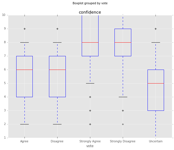
Confidence Grouped by Vote Type
Next, I use the Pandas dataframe grouping function to look at confidence by vote type. Note that the Disagree and Strongly Disagree votes are much less common. Agree is the most common vote, followed by Uncertain and Strongly Agree. Uncertain has the lowest mean confidence at 4.3, possibly because it’s weird to say that you’re ‘confidently uncertain’.
Overall, Strongly Agree and Strongly Disagree have higher mean and median confidences. One possible explanation is that economists are unwilling to step into the Strongly categories unless they feel that they have very good evidence. Another possibility is that this is an issue with the survey – it’s weird to say that you ‘unconfidently strongly agree’.
# Initial grouping, just by vote.

r_list = ['Strongly Disagree', 'Disagree', 'Uncertain', 'Agree', 'Strongly Agree']

filtered_vote = df_responses[df_responses['vote'].isin(r_list)]

filtered_vote.boxplot(column='confidence', by='vote', whis=[5.0,95.0])

df_responses[df_responses['vote'].isin(r_list)].groupby('vote').agg(
                                {'confidence':
                                 {'mean': 'mean',
                                  'std': 'std',
                                  'count': 'count',
'median': 'median'}})| confidence | ||||
|---|---|---|---|---|
| std | count | median | mean | |
| vote | ||||
| Agree | 2.044886 | 2902 | 6 | 5.560992 |
| Disagree | 2.006320 | 992 | 6 | 5.530242 |
| Strongly Agree | 1.764728 | 1347 | 8 | 8.152190 |
| Strongly Disagree | 1.886012 | 314 | 8 | 7.843949 |
| Uncertain | 2.405343 | 1469 | 5 | 4.304969 |
Vote Distance from the Median
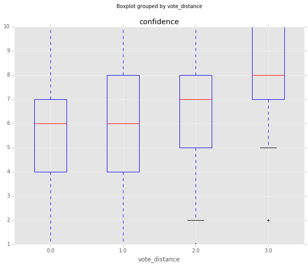
The above results are interesting, but what I’m more interested in is confidence as a claim becomes more controversial. Below, I construct a measure of vote distance from the median vote, then look at confidence grouped by distance from that median. I use the Pandas apply function below to assign a value ranging from 0 (Strongly Disagree) to 4 (Strongly Agree) to both the vote and median_vote columns. I then take the absolute value of the difference between each vote and the median_vote for each question to calculate the distance.
Confidence does increase the further the vote is from the median view, but relationship this is driven by 385 votes two points away, and 25 votes three points away out of a 7024 vote sample. It’s possible that these confident yet controversial votes are from subject matter experts and have more information about a topic than the rest.
def indicator(x):
  if x in r_list:
    return r_list.index(x)
  else:
    return None

df_responses['vote_num'] = df_responses['vote'].apply(indicator)
df_responses['median_num'] = df_responses['median_vote'].apply(indicator)
df_responses['vote_distance'] = abs(df_responses['median_num'] - df_responses['vote_num'])

grouped = df_responses.groupby('vote_distance').agg({'confidence':{'mean': 'mean',
                                                                  'std': 'std',
                                                                  'count':'count'}})


df_responses.boxplot(column='confidence', by='vote_distance', whis=[5.0,95.0]) #bootstrap=1000

grouped| confidence | |||
|---|---|---|---|
| std | count | mean | |
| vote_distance | |||
| 0 | 2.375436 | 3539 | 5.663747 |
| 1 | 2.507784 | 3075 | 6.103089 |
| 2 | 2.429312 | 385 | 6.202597 |
| 3 | 2.406934 | 25 | 7.720000 |
Making a Continuous Vote Column
To add some granularity to the above data, I combine the vote number column and the confidence column into one incremental column called incr_votenum. So a vote of Agree (vote_num = 3) at a confidence of 5 leads to a incr_votenum of 3.454 (3 + 5/11). The assumption I am making here is that confidence is a continuous measure between two votes, with an Agree vote of confidence 10 measuring less than a Strongly Agree vote at confidence 0. I’m not sure if this is a safe assumption to make, but I’m going to run with it.
I then calculate the median incr_votenum for each question, and the distance away from the median for each vote. A few example results are shown in the table below.
# Construct a continuous column, incorporating confidence into vote_num
# Divide by 11 so 10 confidence of agree > 0 confidence of strongly agree
df_responses['incr_votenum'] = df_responses['vote_num'] + df_responses['confidence'] / 11.0

# Median incr_votenum for each question:
df_responses['median_incrvotenum'] = df_responses.groupby(
    ['qtitle','subquestion'])['incr_votenum'].transform('median')

# Calculate distance from median for each econ vote, less biased by outliers.
df_responses['distance_median'] = abs(df_responses['median_incrvotenum'] - \
                                           df_responses['incr_votenum'])

df_responses[df_responses['qtitle'] == 'Brexit II'][
    ['qtitle','subquestion','vote_num','confidence',
'incr_votenum', 'median_incrvotenum', 'distance_median']].head()| qtitle | subquestion | vote_num | confidence | incr_votenum | median_incrvotenum | distance_median | |
|---|---|---|---|---|---|---|---|
| 0 | Brexit II | Question A | 2 | 4 | 2.363636 | 3.363636 | 1.000000 |
| 1 | Brexit II | Question B | 3 | 5 | 3.454545 | 3.272727 | 0.181818 |
| 198 | Brexit II | Question A | 3 | 5 | 3.454545 | 3.363636 | 0.090909 |
| 199 | Brexit II | Question B | 3 | 5 | 3.454545 | 3.272727 | 0.181818 |
| 397 | Brexit II | Question A | 3 | 3 | 3.272727 | 3.363636 | 0.090909 |
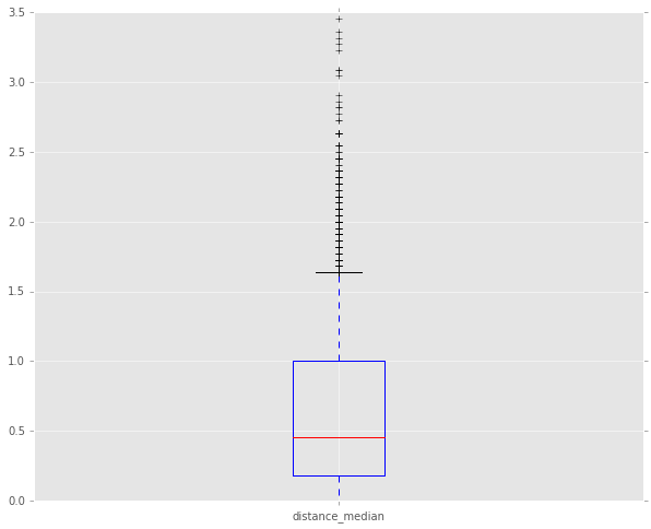
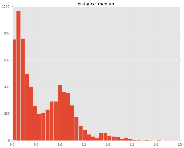
Visualizing the Spread of the Votes
The following boxplot shows the distance from the median for all votes, using the new incremental vote measure. It’s pretty amazing that the mean and median distance away from the consensus are only 0.454 and 0.628 respectively. That’s an impressive amount of consensus. The whiskers on the boxplot cover the 90 percent of the data that fall within roughly 1.6 points of the consensus vote on a scale from 0 to 5.
The histogram also shows a suprising amount of consensus, although it also shows a second peak around a difference of 1.0, which is the difference between two bordering answers, e.g. the distance from Uncertain to Agree.
# Boxplot, showing all vote distances from median
df_responses.boxplot(column='distance_median', whis=[5.0,95.0], return_type='dict')

df_responses.hist(column='distance_median', bins=40)

print 'Median: ' + str(df_responses['distance_median'].median())
print 'Mean: ' + str(df_responses['distance_median'].mean())
print 'Stdev: ' + str(df_responses['distance_median'].std())
Median: 0.454545454545
Mean: 0.628856906192
Stdev: 0.556692286667
Which questions are most controversial?
As a measure of how controversial a question is, I take the standard deviation of the incremental vote number (incr_votenum). I include the final boxplot below, showing the spread of the votes by question.
# Which questions are most controversial?

# Calculating standard deviation, grouped by each question:
grouped_incrvotenum = df_responses.groupby(['qtitle', 'subquestion','qtext'], as_index = False) \
                                        .agg({'incr_votenum': {'std': 'std'}})

# Visualize the spread of responses using a boxplot
qs = grouped_incrvotenum[grouped_incrvotenum.loc[:, ('incr_votenum', 'std')] > 1.05][['qtitle','subquestion']]
qs_most = pd.merge(qs, df_responses, on=['qtitle', 'subquestion'], how='inner')
qs_most.boxplot(column='incr_votenum',by=['qtitle','subquestion'], whis=[5.0,95.0], rot=90) 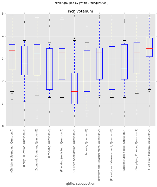
Which questions are least controversial?
# Which questions are least controversial?

# Select all data for questions with qtitle and subquestion by merging
qs_least = grouped_incrvotenum[grouped_incrvotenum.loc[:, ('incr_votenum', 'std')] < 0.6][['qtitle','subquestion']]
qs_least_df = pd.merge(qs_least, df_responses, on=['qtitle', 'subquestion'], how='inner')

# Visualize boxplot and table
qs_least_df.boxplot(column='incr_votenum',by=['qtitle','subquestion'], rot=90, whis=[5.0,95.0]) 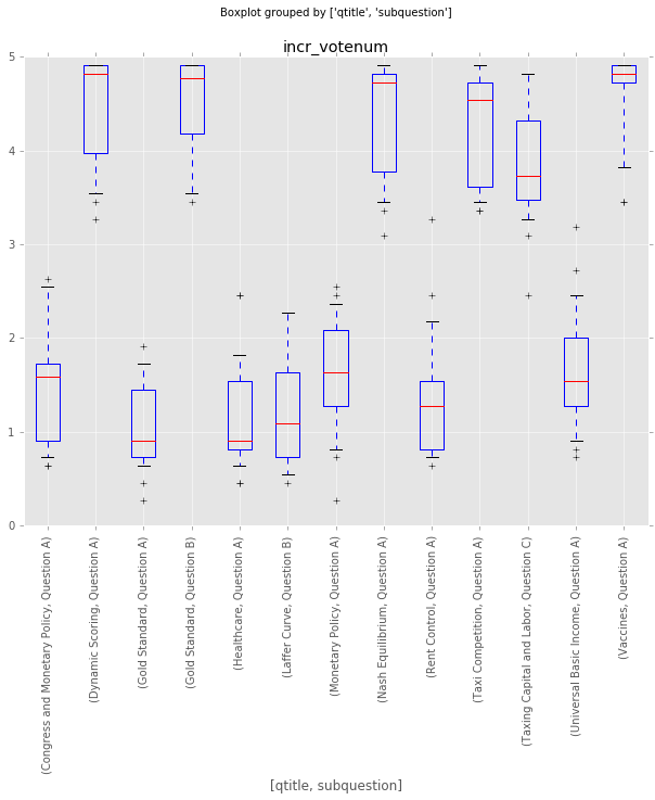
Which economists give more controversial responses?
# Group by economist, calcluate mean distance from median
grouped_econstd = df_responses.groupby(['name', 'institution']).agg({'distance_median': {'mean': 'mean'}})

grouped_econstd[grouped_econstd.loc[:, ('distance_median', 'mean')] > 0.75].sort_values(
                                                                        by=('distance_median','mean'),
ascending=False)| distance_median | ||
|---|---|---|
| mean | ||
| name | institution | |
| Alberto Alesina | Harvard | 0.904429 |
| Angus Deaton | Princeton | 0.891251 |
| Caroline Hoxby | Stanford | 0.889181 |
| Austan Goolsbee | Chicago | 0.791797 |
| Luigi Zingales | Chicago | 0.770085 |
Which economists give the least controversial responses?
# Which economists give the least controversial responses?

grouped_econstd[grouped_econstd.loc[:, ('distance_median', 'mean')] < 0.50].sort_values(
                                                                        by=('distance_median','mean'),
ascending=True)| distance_median | ||
|---|---|---|
| mean | ||
| name | institution | |
| James Stock | Harvard | 0.431818 |
| Amy Finkelstein | MIT | 0.462121 |
| Eric Maskin | Harvard | 0.471361 |
| Raj Chetty | Harvard | 0.474530 |
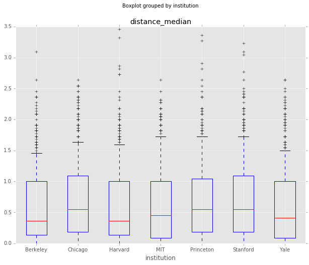
Do any institutions give more controversial responses?
Here’s what Gordon and Dahl had to say about differences between institutions using the 2012 question sample [1, PDF]:
Respondents are dramatically more confident when the academic literature on the topic is large. Not surprisingly, experts on a subject are much more confident about their answers. The middle-aged cohort (the one closest to the current literature) is the most confident, while the oldest (and wisest) cohort is the least confident. Men and those who have worked in Washington do show some tendency to be more confident. Respondents who got their degrees at Chicago are far more confident than the other respondents, with almost as strong an effect for respondents with PhDs from MIT and to a lesser extent from Harvard. Respondents now employed at Yale and to a lesser degree Princeton, MIT, and Stanford seem to be more confident.
It doesn’t seem like any institution sticks out based on this newer data, but maybe with more advanced statistical techniques it might be possible to find something significant.
# Group by institution, calculate mean and stdev of the distance from median response
grouped_inststd = df_responses.groupby(['institution']).agg({'distance_median':
                                                             {'mean': 'mean',
                                                              'std':'std'}}).sort_values(
                                                                        by=('distance_median','mean'),
                                                                        ascending=False)

df_responses.boxplot(column='distance_median', by='institution', whis=[5.0,95.0])

grouped_inststd| distance_median | ||
|---|---|---|
| std | mean | |
| institution | ||
| Stanford | 0.572456 | 0.673072 |
| Chicago | 0.561737 | 0.666043 |
| Princeton | 0.586784 | 0.662991 |
| MIT | 0.554587 | 0.621699 |
| Harvard | 0.558052 | 0.596441 |
| Yale | 0.537219 | 0.593209 |
| Berkeley | 0.526592 | 0.584685 |
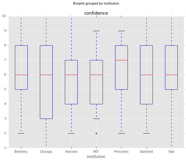
Are any institutions more confident than others?
Again, although there are differences in the mean distance from the consensus view, all the standard deviations overlap, so I don’t think there is anything significant here. Note that Gordon and Dahl also looked at where economists where educated, rather than just where they were employed, and found differences in confidence based on that metric.
#Are any institutions more confident than others?
df_responses.boxplot(column='confidence', by='institution', whis=[5.0,95.0])

grouped_conf = df_responses.groupby(['institution']).agg(
                    {'confidence':
                     {'mean': 'mean',
                      'median':'median',
                      'std':'std'}}).sort_values(by=('confidence','mean'),
                                                     ascending=False)

grouped_conf| confidence | |||
|---|---|---|---|
| std | median | mean | |
| institution | |||
| Princeton | 2.168625 | 7 | 6.363905 |
| Berkeley | 2.360717 | 6 | 6.019286 |
| Yale | 2.457948 | 6 | 6.009033 |
| MIT | 2.094831 | 6 | 5.909300 |
| Stanford | 2.555858 | 6 | 5.859665 |
| Harvard | 2.330881 | 6 | 5.725877 |
| Chicago | 2.789926 | 6 | 5.580745 |
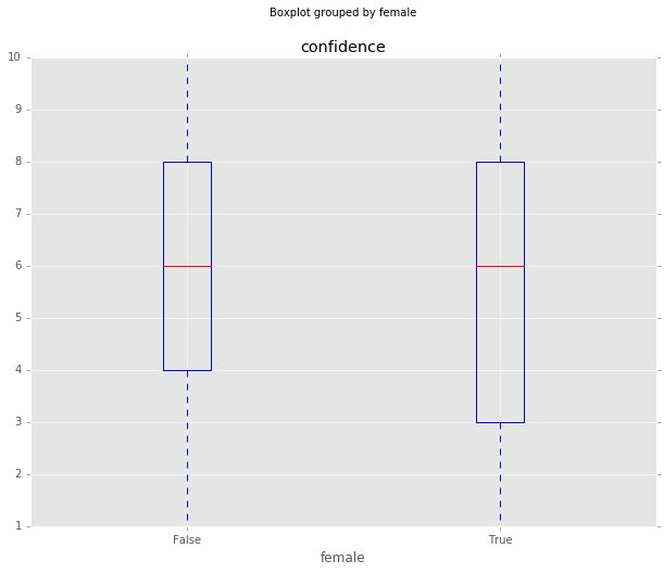
Are male economists more confident?
Gordon and Dahl (2012) noted more confidence among male economists:
The only statistically significant deviation from homogeneous views, therefore, is less caution among men in expressing an opinion, perhaps due to a greater “expert bias.” Personality differences rather than different readings of the existing evidence would then explain these gender effects.
This relationship seems to be less obvious with this expanded dataset. I’m not re-creating their analysis, though, so the difference might still be there if I were to use the controls that they do.
women = ['Amy Finkelstein', 'Hilary Hoynes', 'Pinelopi Goldberg',
         'Judith Chevalier', 'Caroline Hoxby', 'Nancy Stokey',
        'Marianne Bertrand', 'Cecilia Rouse', 'Janet Currie',
         'Claudia Goldin', 'Katherine Baicker']

# Set true/false column based on sex
df_responses['female'] = df_responses['name'].isin(women)

# Boxplot grouped by sex
df_responses.boxplot(column='confidence', by='female', whis=[5.0,95.0])

# Table, stats grouped by sex
df_responses.groupby(['female']).agg({'confidence': {'mean': 'mean', 'std':'std', 'median':'median'}})| confidence | |||
|---|---|---|---|
| std | median | mean | |
| female | |||
| False | 2.398254 | 6 | 5.929568 |
| True | 2.661413 | 6 | 5.729814 |
Conclusion
This is just a first look at the data, and overall there seem to be some pretty interesting patterns. There are probably some other interesting ways to augment this data with other information, like which institution an economist studied at, so I might do that in the future.
Feel free to use the data, let me know what you find!
Sources
[1] Views among Economists: Professional Consensus or Point-Counterpoint? Roger Gordon and Gordon B. Dahl. http://econweb.ucsd.edu/~gdahl/papers/views-among-economists.pdf
[2] Consensus, Polarization, and Alignment in the Economics Profession. Tod S. Van Gunten, John Levi Martin, Misha Teplitskiy. https://www.sociologicalscience.com/articles-v3-45-1028/