Like many people, I’m still recovering from the results of the election. Part of the process for me is coming up with an accurate description of what actually happened, so this post attempts to do so by building a few visualizations.
Building a graphic that clearly communicates the election results is difficult because you need to do a few things simultaneously:
- Use data with enough resolution to show sub-state trends. County level data does a good job here.
- Communicate the size of the vote in each county so we know how consequential it was for the election. If the data is at the national level, weight the vote totals by their contribution to the electoral college.
- Show both the voter turnout and margins for each party. Either can swing an election.
- Compare the outcomes with those of past elections so we can get an idea of what changed this time. Ideally, compare with the average of the past few elections so you’re not comparing against a single candidate or a single point in time.
Below I attempt to accomplish most of those objectives using county level data from Wisconsin. All the code for this post is available in a Jupyter Notebook here, and the data is available in a zipped file here. Update: I also have a new visualization here that does a good job of communicating the 2016 results at the national level.
A Few Examples From Others
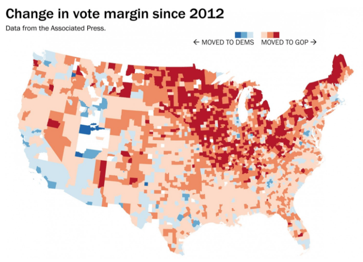
This first example is just a national map, color coding counties by the shift from the 2012 margin. This does a pretty good job of communicating the change since 2012, but I think it over-emphasizes rural counties relative to their population. It also doesn’t communicate anything about changes in turnout, and doesn’t give any idea of the electoral college consequences.
The best graphics I have seen come from a Washington Post article looking at the urban/rural divide, which gets pretty close to meeting all of the above requirements.
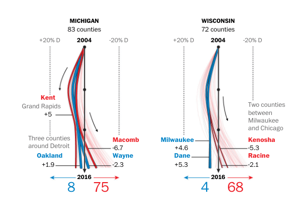
Those graphics are great because they show a smooth change over time and you can get a good overview of what happened relative to the past. The line thickness also gives a good idea of how consequential the county is for vote totals. Unfortunately, this graphic communicates change in voter turnout using line thickness, which makes it difficult to discern differences over time.
Getting the Data For My Own Attempt
I got the county level data for the 2000-2016 elections from David Leip’s Atlas of Presidential Elections. I include a script for getting state level data in the Jupyter notebook.
The voting age population (VAP) data is from the American Community Survey. I downloaded county level data averaged over 2005-2009, and 2010-2014 to try to account for population changes. I calculated turnout by dividing the sum of the votes by the voting age population for each county.
The Final Dataframe
After a lot of data munging, this is the final dataframe. The relevant columns for the graphics are the turnout columns which show the fraction of voting age people that voted in the relevant years, and the dem_lead columns which show the margins between parties for various elections. The demlead_change column shows the difference between the Democratic party lead over the 2000-2012 time period and the lead in 2016.
#Join with turnout_df
turnout_df = pd.merge(turnout_df, spreadall_df, on='county')

#Calculate change in Democratic margin, 2016 - average 2000 to 2012
turnout_df['demlead_change'] = turnout_df['dem_lead_2016'] - turnout_df['dem_lead_2000_2012']

turnout_df.sort_values(by='num_2016', ascending=False, inplace=True)
turnout_df.head(10)| county | num_2016 | turnout_2016 | turnout_2000_2012 | turnout_change | pct_clinton | pct_trump | dem_lead_2016 | num_clinton | num_trump | pct_dem | pct_repub | dem_lead_2000_2012 | demlead_change | |
|---|---|---|---|---|---|---|---|---|---|---|---|---|---|---|
| 40 | Milwaukee | 440698.0 | 0.654155 | 0.703174 | -0.049019 | 65.6 | 28.6 | 37.0 | 288986.0 | 126091.0 | 63.675 | 34.500 | 29.175 | 7.825 |
| 12 | Dane | 309096.0 | 0.830200 | 0.757048 | 0.073152 | 70.4 | 23.1 | 47.3 | 217506.0 | 71270.0 | 67.725 | 29.725 | 38.000 | 9.300 |
| 67 | Waukesha | 237588.0 | 0.808631 | 0.801177 | 0.007454 | 33.3 | 60.0 | -26.7 | 79199.0 | 142519.0 | 33.125 | 65.425 | -32.300 | 5.600 |
| 4 | Brown | 128965.0 | 0.706793 | 0.680866 | 0.025927 | 41.4 | 52.1 | -10.7 | 53358.0 | 67192.0 | 48.150 | 49.975 | -1.825 | -8.875 |
| 44 | Outagamie | 95162.0 | 0.724051 | 0.686042 | 0.038009 | 40.1 | 54.2 | -14.1 | 38117.0 | 51579.0 | 47.750 | 49.950 | -2.200 | -11.900 |
| 51 | Racine | 94921.0 | 0.666838 | 0.686983 | -0.020146 | 44.8 | 49.1 | -4.3 | 42506.0 | 46620.0 | 49.675 | 48.625 | 1.050 | -5.350 |
| 70 | Winnebago | 87140.0 | 0.667714 | 0.678759 | -0.011046 | 42.5 | 49.9 | -7.4 | 37054.0 | 43447.0 | 49.200 | 48.350 | 0.850 | -8.250 |
| 66 | Washington | 77551.0 | 0.776092 | 0.741324 | 0.034768 | 26.9 | 66.7 | -39.8 | 20854.0 | 51729.0 | 30.700 | 67.625 | -36.925 | -2.875 |
| 29 | Kenosha | 76894.0 | 0.636830 | 0.639971 | -0.003141 | 46.5 | 46.9 | -0.4 | 35770.0 | 36025.0 | 54.275 | 43.800 | 10.475 | -10.875 |
| 53 | Rock | 76056.0 | 0.649524 | 0.670892 | -0.021368 | 51.7 | 41.4 | 10.3 | 39336.0 | 31483.0 | 60.050 | 38.150 | 21.900 | -11.600 |
An Initial Attempt
This was my first attempt at a comprehensive plot that meets all the requirements. Average 2000-2012 turnout is on the x-axis, and 2016 turnout is on the y-axis. Any counties above/below the 45 degree line had better/worse turnout in 2016 relative to the average. The area of each of the circles is proportional to the number of votes cast, and the color corresponds with the vote margin.
It’s clear that Milwaukee underperformed in this election. If Milwaukee voted at it’s recent historical average, Wisconsin would probably be a blue state. Unfortunately, this plot doesn’t do good job of communicating the shift in the vote margin relative to the past. For that, I created the next plot.
#http://stackoverflow.com/questions/37401872/custom-continuous-color-map-in-matplotlib
import matplotlib.colors as clr

#Find midpoint of data on 0-1 scale:
vmin = turnout_df['dem_lead_2016'].min()
vmax = turnout_df['dem_lead_2016'].max()
mid = 1 - vmax/(vmax + abs(vmin))

#Construct colormap using midpoint:
cmap = clr.LinearSegmentedColormap.from_list('red_blue',
                        [(0, '#EF3B2C'), (mid, '#FFFFFF'), (1,'#08519C')], N=256)

fig, ax = plt.subplots(figsize=(13,9))

#label='_nolegend_'
plt.scatter(x=turnout_df['turnout_2000_2012'], y=turnout_df['turnout_2016'],
            s=turnout_df['num_2016']/100, marker='o', alpha=1.0, label='Votes',
            c=turnout_df['dem_lead_2016'], cmap=cmap, edgecolors='gray')

ax.set_xlim(0.55, 0.85)
ax.set_ylim(0.55, 0.85)
#s=20

# Create X points
x = pd.DataFrame({'line': np.linspace(0, 1, 100)})
plt.plot(x, x, 'k--', alpha=0.9, label='Equal', color='gray')

A = turnout_df['turnout_2000_2012']
B = turnout_df['turnout_2016']
C = turnout_df['county']
D = turnout_df['num_2016']

for a,b,c,d in zip(A, B, C, D):
    if d > 70000: #Annotate large counties
        ax.annotate('%s' % c, xy=(a,b), textcoords='data')

plt.xlabel('Average Voter Turnout, 2000-2012 (% VAP)')
plt.ylabel('Voter Turnout, 2016 (% VAP)')

legend = plt.legend(loc='upper left')
legend.legendHandles[1]._sizes = [40]

plt.colorbar(shrink=0.5, pad=0.03, label='Democratic Margin', format='%.0f%%')

plt.show()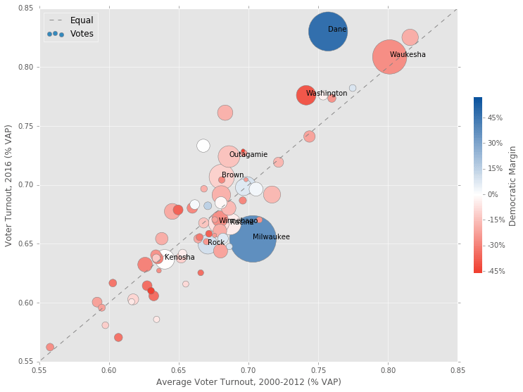
A Better Approach
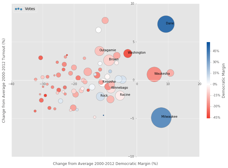
Ok, here is a different approach that matches all of my initial criteria.
It’s easy to build a graphic that shows a difference relative to Obama, but that’s not very informative. Wisconsin has voted for the Democratic nominee in every election since 1984, so Trump’s win should represent a deviation from deeper historical averages, not just a deviation from Obama’s results. That’s what the axes of this graphic try to show, with the x and y axes showing changes from the 2000-2012 averages.
fig, ax = plt.subplots(figsize=(13.5,9))  #figsize=(12,10)

plt.scatter(x=turnout_df['demlead_change'], y=turnout_df['turnout_change']*100,
            s=turnout_df['num_2016']/100, marker='o', alpha=1.0, label='Votes',
            c=turnout_df['dem_lead_2016'], cmap=cmap, edgecolors='gray')

#http://stackoverflow.com/questions/31556446
# Move left y-axis and bottim x-axis to zero:
ax.spines['bottom'].set_position('zero')
ax.spines['left'].set_position('zero')

# Eliminate upper and right axes
ax.spines['right'].set_color('none')
ax.spines['top'].set_color('none')

# Show ticks in the left and lower axes only
ax.xaxis.set_ticks_position('bottom')
ax.yaxis.set_ticks_position('left')

ax.set_ylim(-10, 10)


A = turnout_df['demlead_change']
B = turnout_df['turnout_change']*100
C = turnout_df['county']
D = turnout_df['num_2016']

for a,b,c,d in zip(A, B, C, D):
    if d > 70000: #Annotate large counties  >90000
        ax.annotate('%s' % c, xy=(a,b), textcoords='data')

plt.xlabel('Change from Average 2000-2012 Democratic Margin (%)', labelpad=250)
plt.ylabel('Change from Average 2000-2012 Turnout (%)', labelpad=400)

legend = plt.legend(loc='upper left')
legend.legendHandles[0]._sizes = [40]

#http://stackoverflow.com/questions/5306756
plt.colorbar(shrink=0.5, pad=0.03, label='Democratic Margin', format='%.0f%%') #orientation='horizontal'


plt.show()
So What Happened?
The size and colors of the circles communicate what happened this election. The area of the circle is proportional to the votes cast, and the color shows the margin for the Democrats. It’s pretty easy to get an idea of the crucial counties and the role they played for each party from this data.
The axes in this plot show what changed relative to the past. On the x-axis, I have the change from the average democratic margin, which does a good job of showing the shift in support within a county. This axis makes it clear that there was a massive shift to the Republican party in small rural counties. There was even a shift towards Trump in many larger suburban counties, even if they were still won by Clinton.
Interestingly, Waukesha and Ozaukee counties, which are fairly rich, well educated suburban counties of Milwaukee, actually saw 5-10% shifts towards the Democrats. This fits with Nate Silver’s analysis that suggested level of education was the most important predictor of voting behavior in this election. Waukesha county is one of the most conservative counties in the country, but it’s dominated by establishment conservatives that may have clashed with Trump’s views.
The y-axis shows change in voter turnout relative to the 2000-2012 average. It’s clear that Milwaukee really underperformed here, with a 5% drop in turnout relative to the average. Part of this is probably because Obama wasn’t on the ballot, but the historical average includes the Gore and Kerry elections as well, which should help mitigate the Obama effect.
One thing I haven’t heard anyone discuss is the fact that the Democrat’s margin in Milwaukee was up by 7.8% compared with the 2000-2012 average. A margin increase of 7.8% would lead to a larger net gain in votes than an increase in turnout of the same percent, so this margin increase probably canceled out the effects of lower turnout (although it would be ideal to have increases in both).
Dane County had an amazing 7.3% increase in turnout along with a large 10% increase in Democratic support. This was almost enough to cancel out the poorer performance elsewhere in the state. But in the end, the large shift to Trump in rural counties overwhelmed the Dane County effect.
Why did Dane County do so much better?
Dane County performed much better than Milwaukee County when it comes to voter turnout and margins. It might make sense to try to apply lessons learned from Dane County to Milwaukee, although they are two very different places. There are much higher levels of poverty in Milwaukee, which might magnify the effects of the recent voter ID laws. Anecdotally, there seemed to be less enthusiasm for Clinton as well.
Madison is a younger, more progressive city, and probably had more resources to put into get out the vote efforts. It also has a large student population and one of the top public universities in the world. For more thoughts on the causes of the voting disparities, see this article.
Whatever the cause, I think it makes sense to study the differences between the two counties to look for ways to improve in the future. Things are only going to get more difficult over the coming years with more voter suppression efforts likely at the state and now national level.
Update on Voter ID and Turnout (12/22)
I recently read an interesting paper [1] looking at the effect of Voter ID laws on Democratic and Republican turnout. Until recently, people who have studied voter ID laws haven’t found much effect, but this study was different for a few reasons:
- It used validated voting data. People, especially minority groups, tend to overreport voting behavior in surveys. Using validated data eliminates the problem of inflated turnout by looking at voting records instead.
- Rather than looking at the effect on overall turnout, they looked at the differential effect on minority voters.
- They studied the most recent Photo ID laws, which are more stringent than past laws.
Here’s what they found:
- “The analysis shows that strict photo identification laws have a differentially negative impact on the turnout of Hispanics, Blacks, and mixed-race Americans in primaries and general elections. Voter ID laws skew democracy in favor of whites and those on the political right.”
- “In the general elections, the model predicts Latino turnout was
10.3points lower in states with photo ID than in states without strict photo ID regulations, all else equal. For multi-racial Americans, turnout was12.8points lower under strict photo ID laws.” - “Multi-racial Americans voted at almost the exact same predicted rate as whites (a
0.2point gap) in non-photo ID states but were9.2percent less likely than whites to participate in general elections in photo ID states. Thus, while whites were largely unaffected by these laws, racial and ethnic minorities were falling further and further behind and increasingly losing their place in the democratic process.“ - “Democratic turnout drops by an estimated
7.7percentage points in general elections when strict photo identification laws are in place. By comparison, the predicted drop for Republicans is only4.6points.“
So, if we naively apply these effects to Milwaukee data, what do we see? I don’t have detailed demographic data for the voting population in Milwaukee, so I’ll use the general Democratic (-7.7%) and Republican (-4.6%) effect sizes from above. On the Democratic side, 1.077 x 288,986 = 311,238, an increase of 22,252 votes. For Republicans, 1.046 x 126,091 = 131,891, an increase of 5,800 votes.
Milwaukee turnout was 65.4%, but these additional votes would bring turnout up to (311,238 + 25621 + 131,891)/ (668,249) = 70.1%, which is still below the 2012 turnout of 73.1%. Trump won the state by 22,748 votes, so the increase in Democratic support in Milwaukee County alone would have made things much closer.
If we apply the same Voter ID effects to the rest of the counties in the state using the same approach as above, the result is a 1,489,434 to 1,471,751 Clinton victory. This would bring overall turnout in the state to (1,489,434 + 187320 + 1,471,751)/4,449,170 = 70.8% from 69.6%, which is still in the same ballpark as the 2008 and 2012 elections [2].
The takeaway: if the effect sizes from this paper are correct, the decline in turnout would be enough to swing the election in this state.
Here are a few reasons the above estimate could be wrong:
- The effect size might be smaller in Wisconsin because we might have a smaller minority population than other red states that were included in the study. Using the subgroup specific effects and demographic data from exit polls might be a better approach, but I can’t find a good source for that data. Using the effects by subgroup could also help explain the difference in turnout between Milwaukee County (
60.6%White) and Dane County (84.7%White). - There could be a large overlap of those without a voter ID and those that were uninspired by Clinton as a candidate. Although an ID would have been an impediment, they might not have voted anyways.
- Although the quoted study controlled for many possible confounders, they could be missing one that reduces the effect size.
The results of the above paper have been called into question [3] for data quality issues and some of the problems I mentioned above. The authors haven’t formally issued a response yet, so we’re in “wait and see” mode. This Vox article makes the point that the current body of research shows pretty small effects of ID laws on turnout. But as far as I know, the earlier research hasn’t included more stringent photo ID requirements so it’s likely there isn’t a single “Voter ID Effect”. Instead, the effect probably depends on the context and specific characteristics of the law.
A few political scientists from UW-Madison announced they’re going to study the effects of the law, so it’ll be interesting to compare this back-of-the-envelope estimate with their numbers when they come out next summer. Update: Their study has now been completed. Here’s a summary of the results:
A survey of registered voters in Dane and Milwaukee Counties who did not vote in the 2016 presidential election found that 11.2% of eligible nonvoting registrants were deterred by the Wisconsin’s voter ID law. This corresponds to 16,801 people in the two counties deterred from voting, and could be as high as 23,252 based on the confidence interval around the 11.2% estimate, which is between 7.8% and 15.5%. The survey further found that 6% of nonvoters were prevented from voting because they lacked ID or cited ID as the main reason they did not vote, which corresponds to 9,001 people, and could be as high as 14,101 based on the confidence interval of between 3.5% and 9.4%. Roughly 80% of registrants who were deterred from voting by the ID law, and 77% of those prevented from voting, cast ballots in the 2012 election.
Based on these estimates, if all of the affected registrants voted the voter ID requirement reduced turnout in the two counties by 2.24 percentage points under the main measure of effect, and by 1.2 percentage points under a conservative measure.
So the turnout effects are smaller than in [1], but still substantial enough to flip the state, especially if you found a reasonable way to extrapolate the effects to the rest of the state.
References
[1] Voter Identification Laws and the Suppression of Minority Votes. http://pages.ucsd.edu/~zhajnal/page5/documents/voterIDhajnaletal.pdf
[2] Voter Turnout Estimated at 3.1 million. http://elections.wi.gov/node/4375
[3] Comment on “Voter Identification Laws and the Suppression of Minority Votes” http://stanford.edu/~jgrimmer/comment_final.pdf
[4] Voter ID Study Shows Turnout Effects in 2016 Wisconsin Presidential Election. https://elections.wisc.edu/news/Voter-ID-Study.html, https://elections.wisc.edu/news/Voter-ID-Study/Voter-ID-Study-Release.pdf