This is a second post exploring the data that I collected from the IGM Experts Panel, which surveys a group of leading economists on a variety of policy questions. A CSV of all the data is available here, as are separate datasets of the questions and responses.
One of the interesting things that Gordon and Dahl looked at in their 2012 paper [1, PDF] was how individual characteristics of economists might influence their responses. They compiled information on each economist including the institution of study, graduation year, current university, field of specialization, gender and NBER classification. Ten economists have been added to the group since 2012, so I did my best to gather this information from their CVs and the NBER database. The final CSV of individual characteristics is available here.
Below, I join this dataset of individual characteristics with the responses data from an earlier post, and look at some of the relationships graphically. I don’t have background in economics or a very good understanding of regression analysis, so I stick to plotting trends rather than claiming statistical significance. All of the code for this post is available in an IPython notebook here
Update: A recent study [2] took a look at these data and they make a few important points. First, if the intention of the forum is to show consensus in the economics profession, this might introduce a selection bias towards non-controversial questions. Second, they do find evidence of institutional and political bias but suggest it is a result of the hiring process rather than the educational process.
Loading the Data
Below, I load the data and process it as described in an earlier post. The main result is that I calculate a distance_median column, which is the distance from each response and the median response.
%matplotlib inline

import pandas as pd
import matplotlib.pyplot as plt
import matplotlib
matplotlib.style.use('ggplot')

#pd.set_option('max_colwidth', 30)
pd.set_option('max_colwidth', 400)
matplotlib.rcParams['figure.figsize'] = (10.0, 8.0)

df_responses = pd.read_csv('output_all.csv')
r_list = ['Strongly Disagree', 'Disagree', 'Uncertain', 'Agree', 'Strongly Agree']
def indicator(x):
if x in r_list:
return r_list.index(x)
else:
return None
df_responses['vote_num'] = df_responses['vote'].apply(indicator)
df_responses['median_num'] = df_responses['median_vote'].apply(indicator)
df_responses['vote_distance'] = abs(df_responses['median_num'] - df_responses['vote_num'])
# Construct a continuous column, incorporating confidence into vote_num
# Divide by 11 so 10 confidence of agree > 0 confidence of strongly agree
df_responses['incr_votenum'] = df_responses['vote_num'] + df_responses['confidence'] / 11.0
# Median incr_votenum for each question:
df_responses['median_incrvotenum'] = df_responses.groupby(
['qtitle','subquestion'])['incr_votenum'].transform('median')
# Calculate distance from median for each econ vote, less biased by outliers.
df_responses['distance_median'] = abs(df_responses['median_incrvotenum'] - \
df_responses['incr_votenum'])
df_responses.shape(8402, 18)
Loading and Parsing the Individual Variables
Next, I load and do some processing of the individual variables, getting them into the correct format to join with my responses dataset. I also load in the individual characteristics for the ten new economist, and concatenate those to the original individual characteristics from Gordon and Dahl.
The result of the join is a dataset with 8402 rows and 26 columns.
df_indvars = pd.read_csv('individual-vars.csv')

df_indvars['name'] = df_indvars['name'].str.split(', ').map(lambda row: row[1] + ' ' + row[0])

institutions = ['Berkeley', 'Chicago', 'Harvard', 'MIT', 'Princeton', 'Stanford', 'Yale']

def inst_ind(element):
    return institutions[int(element) - 1]

df_indvars['phdfrom'] = df_indvars['phdfrom'].apply(inst_ind)
df_indvars['currentuniv'] = df_indvars['currentuniv'].apply(inst_ind)


def age_cohort(element):
    cur_year = 116
    cohort = cur_year - int(element)
    if cohort <= 15:
        return '0 - 15 Years'
    elif cohort >= 30:
        return '30+ Years'
    else:
        return '15 - 30 Years'

df_indvars['cohort'] = df_indvars['phdyear'].apply(age_cohort)

ifields = {8:'Industrial Org', 7:'Public Finance', 6:'Labor', 5:'Finance', 4:'Macro', 3:'International'}

def ifield_ind(element):
    return ifields[int(element)]

df_indvars['ifield'] = df_indvars['ifield'].apply(ifield_ind)
# Their coding error?  Alesina is listed as MAC in appendix, but has ifield of 3?
# df_indvars[]  change it?

# Load individual variables from 10 new economists
# Self coded based on personal websites, NBER information
# http://www.nber.org/programs/
df_indvarsnew = pd.read_csv('individual_vars_new.csv')

# Add cohort column
df_indvarsnew['cohort'] = df_indvarsnew['phdyear'].apply(age_cohort)

# Concat both old and new individual vars datasets
df_indvarsall = pd.concat([df_indvars, df_indvarsnew], ignore_index=True)

#df_indvarsall.to_csv('indvars_2016.csv', encoding='utf-8', index=False)

df_indvarsall.head()

# Gordon Online Appendix and Data:
# http://econweb.ucsd.edu/~gdahl/views-among-economists-code.html
# http://econweb.ucsd.edu/~gdahl/papers/views-among-economists-online-appendix.pdf
# Notes: PhD From and Current University categories are BER=Berkeley; CHI=Chicago, Rochester; HAR=Harvard,
#     Cambridge, LSE, Wisconsin; MIT=MIT, Oxford; PRI=Princeton; STA=Stanford; YAL=Yale.
#     Field categories are defined by primary NBER affiliation: MAC=macro (EFG, ME, POL); INT=international (IFM, ITI);
#         FIN=finance (AP, CF); LAB=labor (LS, ED, AG, DAE, DEV); PF=public finance (PF, EEE);
#         IO=industrial organization (IO, LE). Three panel members are not in the NBER;
#         Ray Fair and James Stock are assigned to MAC, Eric Maskin is assigned to FIN.
# Female is an indicator equal to 1 for women. Wash is an indicator for experience serving in Washington.| name | phdyear | phdfrom | currentuniv | ifield | gender | washington | nber | cohort | |
|---|---|---|---|---|---|---|---|---|---|
| 0 | Daron Acemoglu | 92 | Harvard | MIT | Labor | 1 | 0 | LS | 15 - 30 Years |
| 1 | Alberto Alesina | 86 | Harvard | Harvard | International | 1 | 0 | POL | 30+ Years |
| 2 | Joseph Altonji | 81 | Princeton | Yale | Labor | 1 | 0 | LS | 30+ Years |
| 3 | Alan Auerbach | 78 | Harvard | Berkeley | Public Finance | 1 | 1 | PE | 30+ Years |
| 4 | David Autor | 99 | Harvard | MIT | Labor | 1 | 0 | LS | 15 - 30 Years |
# Inner join, on name column
df_all = pd.merge(df_responses, df_indvarsall, on=['name'], how='inner')

print df_all.shape
# Remove middle initials for Brunnermeier, Kaplan, to get right shape of (8402, 26)
(8402, 26)
Confidence by Education
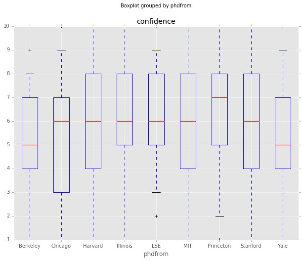
One of the interesting things Gordon and Dahl found was that economists that were educated at MIT and the University of Chicago seemed to be more confident. I find less evidence of this in the newer data, although this is just a boxplot, not a regression analysis.
df_all.boxplot(column='confidence', by='phdfrom', whis=[5.0,95.0])

df_all.groupby('phdfrom').agg({'confidence':{'mean': 'mean', 'median':'median',
                                            'std': 'std', 'count':'count'}}).sort_values(
                                                                        by=('confidence','mean'),
ascending=False)| confidence | ||||
|---|---|---|---|---|
| std | count | median | mean | |
| phdfrom | ||||
| LSE | 1.964802 | 93 | 6 | 6.290323 |
| MIT | 2.494196 | 2414 | 6 | 6.063380 |
| Princeton | 2.404093 | 591 | 7 | 6.000000 |
| Illinois | 2.839723 | 112 | 6 | 5.910714 |
| Stanford | 2.430876 | 959 | 6 | 5.851929 |
| Harvard | 2.384803 | 2082 | 6 | 5.850144 |
| Yale | 2.399019 | 358 | 5 | 5.410615 |
| Chicago | 2.538058 | 387 | 6 | 5.395349 |
| Berkeley | 2.310260 | 28 | 5 | 5.178571 |
Distance from Median by Education
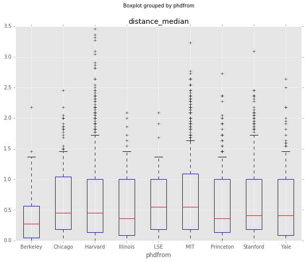
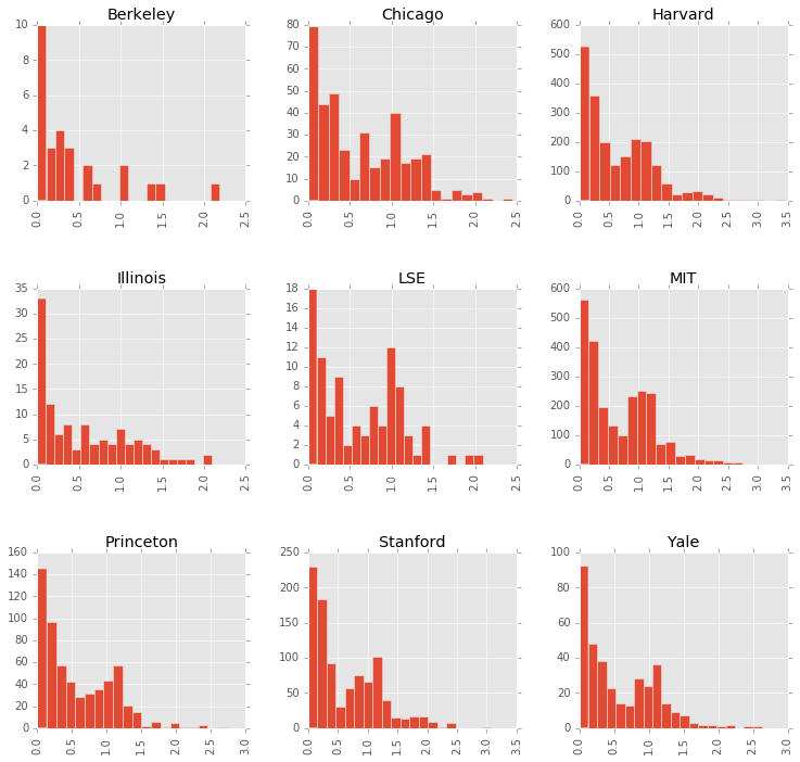
Another interesting thing to look at is whether any institutions produce graduates with views further from the median view. There definitely are differences in the means and medians below, but I don’t think they would rise to the level of significance because the standard deviations overlap.
It’s also important to note that the vote counts by institution vary from 2414 (MIT) to 28 (Berkeley), so these responses don’t represent the institution as a whole.
df_all.boxplot(column='distance_median', by='phdfrom', whis=[5.0,95.0])

df_all.hist(column='distance_median', by='phdfrom', bins=20, figsize=(12,12))

df_all.groupby('phdfrom').agg({'distance_median':{'mean': 'mean', 'median':'median',
                                            'std': 'std', 'count':'count'}}).sort_values(
                                                                        by=('distance_median','mean'),
                                                                        ascending=False)

#Only 28 votes from Berkeley
#len(df_all[(df_all['phdfrom'] == 'Berkeley') & (df_all['vote'].isin(r_list))])| distance_median | ||||
|---|---|---|---|---|
| std | count | median | mean | |
| phdfrom | ||||
| MIT | 0.559621 | 2414 | 0.545455 | 0.655363 |
| Harvard | 0.580161 | 2082 | 0.454545 | 0.638023 |
| Chicago | 0.524551 | 387 | 0.454545 | 0.633427 |
| LSE | 0.489293 | 93 | 0.545455 | 0.621701 |
| Stanford | 0.559780 | 959 | 0.409091 | 0.621149 |
| Yale | 0.522308 | 358 | 0.409091 | 0.574022 |
| Princeton | 0.501498 | 591 | 0.363636 | 0.556145 |
| Illinois | 0.523816 | 112 | 0.363636 | 0.551542 |
| Berkeley | 0.536900 | 28 | 0.272727 | 0.431818 |

Washington Insiders
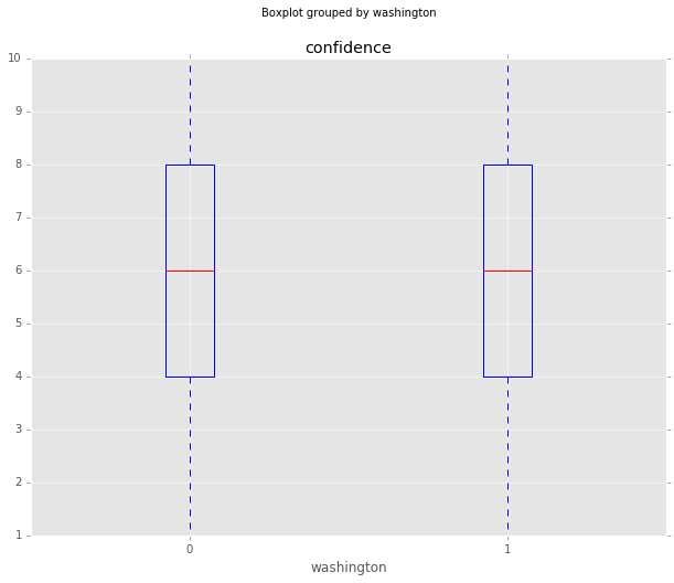
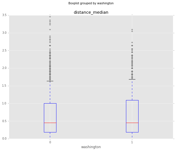
Spending time in Washington doesn’t seem to have much of an effect on confidence. Those that haven’t spent time in Washington maybe have a little bit longer tail when it comes to controversial responses, but overall both groups are very similar.
df_all.boxplot(column='confidence', by='washington', whis=[5.0,95.0])

df_all.boxplot(column='distance_median', by='washington', whis=[5.0,95.0])
<matplotlib.axes._subplots.AxesSubplot at 0x107292790>
How do responses differ by field of study?
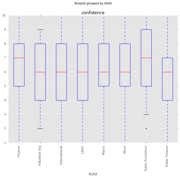
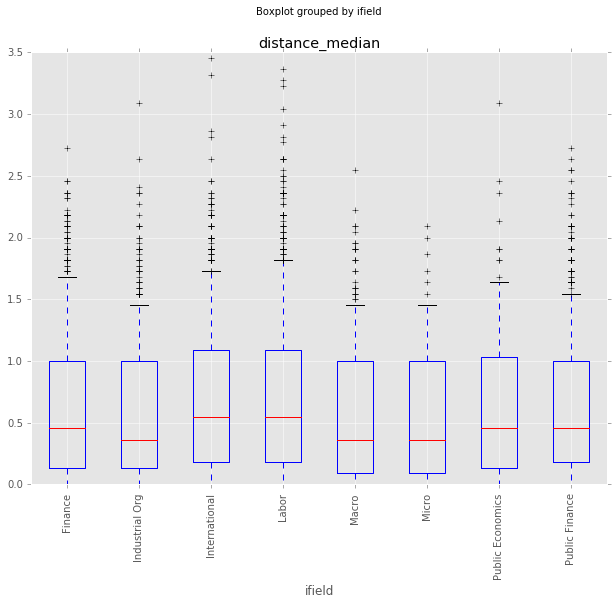
Gordon and Dahl also used the NBER classification of each economist to look at how responses changed by field of study. I do something similar below, looking at confidence and distance_median grouped by field of study. The Finance and Public Economics groups seem a little more confident. The International and Labor Economics groups seem to have a little higher distance_median, but it’s unlikely any of this rises to the level of significance.
# http://econweb.ucsd.edu/~gdahl/papers/views-among-economists-online-appendix.pdf
# ifield is grouped nber classifications:
#     Field categories are defined by primary NBER affiliation: MAC=macro (EFG, ME, POL); INT=international (IFM, ITI);
#         FIN=finance (AP, CF); LAB=labor (LS, ED, AG, DAE, DEV); PF=public finance (PF, EEE);
#         IO=industrial organization (IO, LE). Three panel members are not in the NBER;
#         Ray Fair and James Stock are assigned to MAC, Eric Maskin is assigned to FIN.

df_all.boxplot(column='confidence', by='ifield', rot=90, whis=[5.0,95.0])

df_all.boxplot(column='distance_median', by='ifield', rot=90, whis=[5.0,95.0])
<matplotlib.axes._subplots.AxesSubplot at 0x1039ccd50>
Responses by Age Cohort
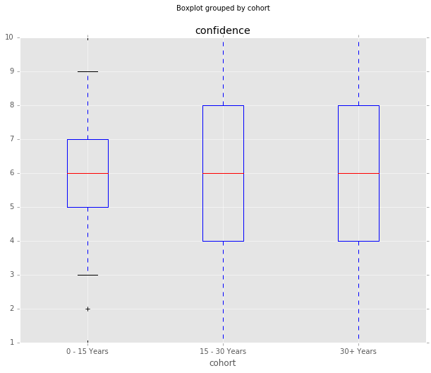
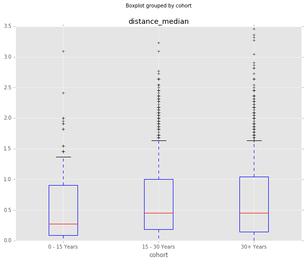
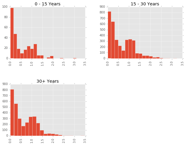
One final thing to do is look at these characteristics by age cohort, defined as years since their PhD. Confidence doesn’t seem to be too different by age cohort, but it does seem like there are more outlier responses in the older groups. Perhaps the older economists have earned the right to say controversial things?
df_all.boxplot(column='confidence', by='cohort', whis=[5.0,95.0])

df_all.boxplot(column='distance_median', by='cohort', whis=[5.0,95.0])

df_all.hist(column='distance_median', by='cohort', bins=20)

df_all.groupby('cohort').agg({'distance_median':{'mean': 'mean', 'median':'median',
                                            'std': 'std', 'count':'count'},
                             'confidence': {'mean': 'mean', 'median':'median',
                                            'std': 'std'}}).sort_values(by=('distance_median','mean'),
ascending=False)| distance_median | confidence | ||||||
|---|---|---|---|---|---|---|---|
| std | count | median | mean | std | median | mean | |
| cohort | |||||||
| 30+ Years | 0.561107 | 3230 | 0.454545 | 0.633971 | 2.413021 | 6 | 6.013622 |
| 15 - 30 Years | 0.554432 | 3510 | 0.454545 | 0.632673 | 2.503507 | 6 | 5.789744 |
| 0 - 15 Years | 0.524708 | 284 | 0.272727 | 0.523528 | 2.111850 | 6 | 5.795775 |
Conclusion
Ok, that’s it for now. There do seem to be some interesting patterns in this data, but I’m not sure if any rise to the level of statistical significance. I guess I have to learn the regression techniques economists use to say anything further.
Thanks for reading, and let me know if you have any comments or questions.
Sources
[1] Views among Economists: Professional Consensus or Point-Counterpoint? Roger Gordon and Gordon B. Dahl. http://econweb.ucsd.edu/~gdahl/papers/views-among-economists.pdf
[2] Consensus, Polarization, and Alignment in the Economics Profession. Tod S. Van Gunten, John Levi Martin, Misha Teplitskiy. https://www.sociologicalscience.com/articles-v3-45-1028/