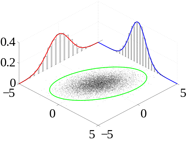
I recently worked on a visualization where I needed to draw numbers from a joint probability distribution. This ended up being much harder than I thought it would be, so I thought I’d write up the results to save someone else some time. There are a number of resources out there for doing this in languages like Python and R, but nothing for JavaScript. I ended up using jStat for many of it’s distributions and helper functions, along with this Stackoverflow answer.

Here are the steps:
- Create uncorrelated samples drawing from a standard normal distribution (mu=0, sigma=1).
- Create a correlation matrix with the desired correlation between the samples.
- Matrix multiply the cholesky decomposition of the correlation matrix with the uncorrelated samples to create correlated normal samples.
- Convert the correlated normal samples to correlated uniform samples using the standard normal cumulative distribution function (CDF). I think the result of this is considered a copula.
- Use the inverted CDF of the desired distributions to convert the correlated uniform samples into correlated samples. This is called inverse transform sampling.
Note that the sample correlation won’t be exactly what you specified in the correlation matrix, but it was close enough for my purposes. If you need a specific correlation, you could always write a while loop that repeats this process until it’s within a certain threshold of your desired correlation. Here’s the code for a joint lognormal distribution:
//script src="https://cdn.jsdelivr.net/npm/jstat@latest/dist/jstat.min.js" /script

function generateCopula(rows, columns, correlation) {
    //https://en.wikipedia.org/wiki/Copula_(probability_theory)

    //Create uncorrelated standard normal samples
    var normSamples = jStat.randn(rows, columns);

    //Create lower triangular cholesky decomposition of correlation matrix
    var A = jStat(jStat.cholesky(correlation));

    //Create correlated samples through matrix multiplication
    var normCorrSamples = A.multiply(normSamples);

    //Convert to uniform correlated samples over 0,1 using normal CDF
    var normDist = jStat.normal(0,1);
    var uniformCorrSamples = normCorrSamples.map(function(x) {return normDist.cdf(x);});

    return uniformCorrSamples;

}

function generateCorrLognorm(number, mu, sigma, correlation) {

    //Create uniform correlated copula
    var copula = generateCopula(mu.length, number, correlation);

    //Create unique lognormal distribution for each marginal
    var lognormDists = [];
    for (var i = 0; i < mu.length; i++) {
        lognormDists.push(jStat.lognormal(mu[i], sigma[i]));
    }

    //Generate correlated lognormal samples using the inverse transform method:
    //https://en.wikipedia.org/wiki/Inverse_transform_sampling
    var lognormCorrSamples = copula.map(function(x, row, col) {return lognormDists[row].inv(x);});
    return lognormCorrSamples;
}

var mu = [0,0],
	sigma = [0.25, 0.5],
	correlation = [[1.0, 0.5],[0.5, 1.0]];

var data  = generateCorrLognorm(100, mu, sigma, correlation);
A nice feature of this approach is that you can use any combination of distributions and create any number of correlated samples. All you need is to do is create the desired correlation matrix, define the distributions with jStat, and then use their inverted CDFs to convert the copula.
For example, if I wanted a joint normal-lognormal distribution, I could use the copula function above, then independently define distributions and use their inverted CDFs:
var rows = 2,   //number of distributions
    columns = 100;  //number of samples
    correlation = [[1.0, 0.5],[0.5, 1.0]];

var copula = generateCopula(rows, columns, correlation);

var normal = jStat.normal(0, 1),
    lognormal = jStat.lognormal(0, 0.5),
    dists = [normal, lognormal];

var samples = copula.map(function(x, row, col) {return dists[row].inv(x);});
Note that the map function used above is unique to jStat because it can operate across multiple arrays. The samples variable above is now an array with two correlated samples, one with a normal distribution and one with a lognormal one:
> samples
[[-0.3111414911440098, -0.020000657895910958, -0.753150640735201, 0.45079960956056986, ...],
 [0.7902422132853483, 1.589785300759001, 0.6259310681427537, 0.8549897874735056, ...]]