Synthetic populations are created to represent demographic and geographic data for a population without revealing the underlying data for any individuals. This is done by using an iterative proportional fitting technique to create fake individuals and households that, when aggregated, match the characteristics of each census tract. I recently came across a synthetic population for the entire US on the Pitt Public Health Dynamics Lab website, so I decided to download and experiment with it:
Synthetic populations are traditionally used for things like epidemic modeling and emergency response planning, but they could also be used for something else: calculating voter demographic and turnout data for state legislative districts. I couldn’t do this in the past because the Census Bureau doesn’t release data subdivided by state legislative districts (as far as I can tell). But now that I have a synthetic population, all I need to do is write an SQL query to get the data I need. In addition, I can ask questions like “Which state legislative district has the most voters under 30 with an income of less than $30,000?”, a level of detail that’s impossible to get from the Census data alone.
Below I show all the steps for getting started with the data with Postgres, PostGIS and Python. At the end, I write an SQL query that finds the voting age population for all the Wisconsin State Assembly districts in 2016. All the code for this post is available on GitHub here.
Setting up the Database
If you don’t have Postgres or Postgis installed this can be done from the command line if you use brew on a mac:
$ brew update
$ brew install postgresql
$ brew install postgis
$ brew services start postgresql
Then use these bash commands to create the database and add the postgis extension:
$ createdb -U psthomas synthpop
$ psql -U psthomas -d synthpop -c "CREATE EXTENSION postgis"
Also, set your user password, and export it into the environment for use later:
$ export POSTGRESPASS='<your-postgres-pass>'Importing the Geography Data
This next step can be done on the commmand line as well with ogr2ogr, a command line utility for converting between geospatial data types. In this case, I’m converting an ESRI geodatabase (.gdb) into a Postgres database. This could be automated as a shell script, but I found it easiest to just use the command line.
First, find the geodatabase that’s relevant to your analysis on the Census Bureau website. Download it, then use ogrinfo to find the names of the different tables available:
$ ogrinfo "/Volumes/Misc/projects/snythpop/data/geographies/tlgdb_2019_a_us_legislative.gdb.zip"
INFO: Open of `/Volumes/Misc/projects/synthpop/data/geographies/tlgdb_2019_a_us_legislative.gdb.zip'
      using driver `OpenFileGDB' successful.
1: Congressional_Districts_116th (Multi Polygon)
2: State_Legislative_Districts_Upper (Multi Polygon)
3: State_Legislative_Districts_Lower (Multi Polygon)
4: Voting_Districts (Multi Polygon)
Next, use ogr2ogr to load the desired geography table into the Postgres database you set up above. In this case I’m loading the shapes for the lower state legislative districts (State_Legislative_Districts_Lower). Note that I’m using the POSTGRESPASS environmental variable that we exported earlier for the password.
$ ogr2ogr -overwrite -skipfailures -f "PostgreSQL" PG:"host=localhost user=psthomas dbname=synthpop password=$POSTGRESPASS" "/Volumes/Misc/projects/synthpop/data/geographies/tlgdb_2019_a_us_legislative.gdb.zip" "State_Legislative_Districts_Lower"And here’s a similar command loading the urban area outlines for the Milwaukee dot plot later:
$ ogr2ogr -overwrite -skipfailures -f "PostgreSQL" PG:"host=localhost user=psthomas dbname=synthpop password=$POSTGRESPASS" "/Volumes/Misc/projects/synthpop/data/geographies/tlgdb_2019_a_us_nationgeo.gdb.zip" "Urban_Area"Note that I’m also loading the data directly from the zipped files because the files were unreadable if unzipped on my computer for some reason. Repeat these steps until you have all the geography tables you need for your analysis.
Importing the Synthetic Population
The next step is to download and import the synthetic population data. I found the synthetic population data on the Pitt Public Health Dynamics Lab website, with the population originally developed by RTI International as a part of the Models of Infectious Disease Agency Study (MIDAS). I manually downloaded the data for each state, extracted the files, and then used the code below to create tables and load the data. Note that the files are vey large (>30GB extracted), so you might want to put the data on an external drive.
From here on out, all the code is written in Python, with the SQL queries handled by psycopg2. You can see all the code for this post available in a Jupyter Notebook here. First we need to import all the project dependencies, which include Pandas, Numpy, and GeoPandas.
import os
import glob
from pathlib import Path
import numpy as np
import pandas as pd
import geopandas as gpd
import psycopg2
from IPython.display import display
import matplotlib.pyplot as plt
import matplotlib
Next, we make a connection with the database we created earlier using psycopg2:
pw = os.environ['POSTGRESPASS'] # Password from current environment
connection = psycopg2.connect(database="synthpop", user="psthomas", password=pw)
cursor = connection.cursor()
After connecting to the database, we need to create create the tables along with their schemas. This is handled below:
cursor.execute('''
DROP TABLE IF EXISTS households;
''')

# Creating the households table
cursor.execute('''
CREATE TABLE households (
sp_id VARCHAR,
stcotrbg VARCHAR,
hh_race BIGINT,
hh_income BIGINT,
latitude DOUBLE PRECISION,
longitude DOUBLE PRECISION,
coordinate geometry);
''')

connection.commit()

# Creating the people table
cursor.execute('''
DROP TABLE IF EXISTS people;
''')

cursor.execute('''
CREATE TABLE people (
sp_id VARCHAR,
sp_hh_id VARCHAR,
age BIGINT,
sex VARCHAR,
race BIGINT,
relate BIGINT,
school_id VARCHAR,
work_id VARCHAR);
''')

connection.commit()
Now that we have the tables created, they’re ready to accept the data. In this first step, I recursively search through the synthetic population directories for all the households.txt files, which contain households along with their latitudes and longitudes. I then iterate through these files, copying them into the households table. Note that I’m only loading the data for Wisconsin for now – loading the rest of the data takes up all the disk space on my little old Macbook Air, so I need to move to the cloud if I want query the entire population.
filepath = os.path.join(os.getcwd(), 'data', 'synthpops', 'WI')

# Delete any existing data first
cursor.execute("DELETE FROM households")

for f in Path(filepath).rglob('households.txt'):
    sql = '''
    COPY households(sp_id, stcotrbg, hh_race, hh_income, latitude, longitude)
    FROM '{0}' DELIMITER '  ' CSV HEADER;
    '''.format(f)
    cursor.execute(sql)

# Commit the results
connection.commit()
The next step is to convert the latitude/longitude columns into a Point geometry in PostGIS. The documentation on the synthetic population says it was created using the World Geodetic System of 1984 (srid = 4326), so that’s what I specify when I create the points.
cursor.execute('''
UPDATE households
SET coordinate = ST_GeomFromText('POINT(' || longitude || ' ' || latitude || ')', 4326);
''')
There’s a problem with these points though: this coordinate system is different from the one that the Census Bureau uses (srid = 4269), so all these points need to be transformed in order to do spatial queries on them. This is done below:
cursor.execute('''
UPDATE households
SET coordinate = ST_Transform(coordinate, 4269);
''')

# Commit the results
connection.commit()
Ok, so now we have all of our households geocoded and transformed into the right coordinate system. Next, we need to load all of the people, which can be connected to the households via the sp_hh_id column. Luckily, there are no geography columns to worry about here, so this step is easier:
# Delete existing data first
cursor.execute("DELETE FROM people")

for f in Path(filepath).rglob('people.txt'):
    sql = '''
    COPY people(sp_id, sp_hh_id, age, sex, race, relate, school_id, work_id)
    FROM '{}' DELIMITER '   ' CSV HEADER;
    '''.format(f)
    cursor.execute(sql)

# Commit the results
connection.commit()
Great, now we have all of our people and household data loaded. The final thing to do is to add indexes to a few columns to speed up the joins. This is especially important for spatial data because it uses bounding boxes to greatly limit the number of comparisons that need to be made during spatial joins.
# Create an index on coordinates.
# Still useful for coordinates because it uses RTree data structure
# https://gis.stackexchange.com/questions/265966
# https://postgis.net/workshops/postgis-intro/indexing.html
cursor.execute('''
CREATE INDEX house_geometry_index
ON households
USING GIST(coordinate);
''')

# Create an index on sp_id for faster joins
# https://www.postgresql.org/docs/11/indexes-intro.html
cursor.execute('''
CREATE INDEX house_id_index
ON households (sp_id);
''')

# Create an index on sp_hh_id for faster join onto households sp_id
# https://www.postgresql.org/docs/11/indexes-intro.html
cursor.execute('''
CREATE INDEX person_house_id_index
ON people (sp_hh_id);
''')
All of the Census boundaries that we loaded earlier with ogr2ogr already have spatial indexes, so we don’t need to worry about adding those. Alright, we finally have all of the data loaded and prepared for querying!
Here is a list of the tables we now have available in our synthpop database:
synthpop=# \dt
                       List of relations
 Schema |               Name                | Type  |  Owner
--------+-----------------------------------+-------+----------
 public | households                        | table | psthomas
 public | people                            | table | psthomas
 public | spatial_ref_sys                   | table | psthomas
 public | state_legislative_districts_lower | table | psthomas
 public | urban_area                        | table | psthomas
A Dotmap of Milwaukee
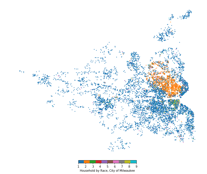
To start out with a simple query, I thought it would be interesting to create a dotmap of my hometown of Milwaukee. The households table has a column for race, so we can use that to get a good idea of the demographics of different parts of the city.
The query below is a fairly standard select statement but with a twist – the ST_Contains(u.shape, h.coordinate) statement. This functionality is added by PostGIS, and it allows you to select the geometries fully contained within another geometry (in this case, the households within the Milwaukee urban area). I then randomly select 10,000 households using the ORDER BY random() LIMIT 10000 clause. Getting this data into Python is then as simple as passing this query and the connection to the GeoPandas from_postgis function. Pretty nice!
dot_query = '''
SELECT
    u.geoid,
    h.sp_id,
    h.coordinate,
    h.hh_race
FROM households AS h
    JOIN urban_area AS u
    ON ST_Contains(u.shape, h.coordinate)
WHERE u.geoid = '57466'
ORDER BY random()
LIMIT 10000;
'''

dot_df = gpd.GeoDataFrame.from_postgis(dot_query, connection, geom_col='coordinate')
display(dot_df.head())| geoid | sp_id | coordinate | hh_race | |
|---|---|---|---|---|
| 0 | 57466 | 54323919 | POINT (-88.06619 43.05997) | 9 |
| 1 | 57466 | 55191668 | POINT (-88.21111 42.98681) | 1 |
| 2 | 57466 | 53797371 | POINT (-87.99648 43.02619) | 1 |
| 3 | 57466 | 53779988 | POINT (-87.98308 43.07194) | 2 |
| 4 | 57466 | 55637265 | POINT (-88.18592 43.20900) | 1 |
Next, I need to map this. GeoPandas has some great built-in mapping functionality, so let’s use that.
# http://geopandas.org/mapping.html
fig, ax = plt.subplots(figsize=(12,12))

dot_df.plot(ax=ax, column='hh_race', legend=True, markersize=2, cmap='tab10',
    legend_kwds={'label': "Household by Race, City of Milwaukee",
    'orientation': 'horizontal','pad':0.01,'shrink':0.3})
ax.axis('off')

plt.show()
And there we go, we can clearly see the racial demographics of the Milwaukee area. The blue dots are White households, the orange dots are Black households, and green dots are Other (mostly Hispanic on the south side of Milwaukee in this case). Milwaukee is one of the most segregated cities in the country so, although regrettable, these patterns show up pretty clearly.
2016 Turnout, Wisconsin State Assembly
I mentioned at the beginning that I wanted to calculate the voter turnout for the 2016 Wisconsin State Assembly districts, so let’s do that next. As far as I can tell, the Census Bureau doesn’t release their data broken down by state legislative districts, so having a synthetic population makes this previously-impossible analysis possible.
The query below is more complex, but I tried to simplify it by breaking it up into common table expressions (CTE). The first CTE uses the state legislative outlines and the ST_Contains function to find the district for each household. The second CTE joins the people table onto the households table and then groups and sums the people (age 18+) by geoid, making a voting age population column. Finally, this data is joined back onto the legislative outlines table and returned to GeoPandas for plotting purposes. The end result is a count of the voting age population for each district derived entirely from a synthetic population.
query = '''
WITH lower_households AS (
SELECT
    s.geoid,
    h.sp_id,
    h.coordinate
FROM households AS h
    JOIN state_legislative_districts_lower AS s
    ON ST_Contains(s.shape, h.coordinate)
WHERE s.geoid LIKE '55%'
),
wisclower_vap AS (
SELECT
    geoid,
    count(p.sp_id) AS voting_age_pop
FROM people AS p
    JOIN lower_households AS l
    ON l.sp_id = p.sp_hh_id
WHERE p.age >= 18
GROUP BY l.geoid
ORDER BY voting_age_pop DESC)

SELECT
    w.geoid,
    w.voting_age_pop,
    s.shape
FROM wisclower_vap AS w
    JOIN state_legislative_districts_lower as s
    ON w.geoid = s.geoid
LIMIT 1000;
'''

poly_df = gpd.GeoDataFrame.from_postgis(query, connection, geom_col='shape')
poly_df.head()| geoid | voting_age_pop | shape | |
|---|---|---|---|
| 0 | 55001 | 44343 | MULTIPOLYGON (((-87.94429 44.67813, -87.93753 ... |
| 1 | 55002 | 41595 | MULTIPOLYGON (((-88.12635 44.46920, -88.12572 ... |
| 2 | 55003 | 42106 | MULTIPOLYGON (((-88.16546 44.13169, -88.16546 ... |
| 3 | 55004 | 42937 | MULTIPOLYGON (((-88.14988 44.50133, -88.14845 ... |
| 4 | 55005 | 41751 | MULTIPOLYGON (((-88.19132 44.33248, -88.19131 ... |
Note that this computation takes about ten minutes on my old Macbook Air (1.6GHz, 4GB Ram), so I would need to use a cloud server to perform the computation for state legislatures across the entire nation. The next step is to merge this data with Wisconsin Assembly election results from a previous analysis to calculate turnout and margins:
# Elections Data from a previous analysis: https://pstblog.com/2019/03/05/voting-power-comprehensive
results_path = os.path.join(os.getcwd(), 'data', 'election_results', 'state_house.csv')
results_df = pd.read_csv(results_path)

final_df = poly_df.merge(results_df[['geoid','totalvote', 'dem_margin']], on='geoid')
final_df['turnout'] = (final_df['totalvote']/final_df['voting_age_pop'])*100
final_df['rep_margin'] = -1*final_df.dem_margin
final_df[['geoid', 'shape', 'voting_age_pop', 'totalvote', 'rep_margin', 'turnout']] \
.sort_values(by='turnout', ascending=False).head(5)| geoid | shape | voting_age_pop | totalvote | rep_margin | turnout | |
|---|---|---|---|---|---|---|
| 73 | 55076 | MULTIPOLYGON (((-89.42083 43.06248, -89.42054 ... | 45667 | 40505.0 | -66.043698 | 88.696433 |
| 11 | 55014 | MULTIPOLYGON (((-88.18598 43.08239, -88.18597 ... | 43184 | 34935.0 | 14.504079 | 80.898018 |
| 76 | 55079 | MULTIPOLYGON (((-89.26300 43.10712, -89.26200 ... | 46805 | 36316.0 | -27.827955 | 77.590001 |
| 53 | 55056 | MULTIPOLYGON (((-88.88675 44.24121, -88.88674 ... | 42228 | 32573.0 | 29.076229 | 77.136023 |
| 35 | 55038 | MULTIPOLYGON (((-88.80975 43.02505, -88.80962 ... | 42995 | 32996.0 | 25.518245 | 76.743807 |
State Assembly District 76 (geoid 55076) has the highest turnout (88.7%), which makes sense because it includes the state capitol building in Madison. I guess people are pretty politically engaged around those parts. The final step is to create a few visualizations of the results using the GeoPandas built in mapping features again. Here’s the margin by district:
plot_df = final_df.copy()
plot_df['rep_margin'] = plot_df['rep_margin'].clip(lower=-25.0, upper=25.0)
#Change coordinate system for a more legible map
#https://spatialreference.org/ref/epsg/2288/
plot_df = plot_df.to_crs({'init': 'EPSG:2288'})

fig, ax = plt.subplots(figsize=(12,11))
ax.axis('off')
plot_df.plot(ax=ax, column='rep_margin', linewidth=0.1, cmap='coolwarm',legend=True,
    legend_kwds={'label': "Republican Margin, 2016 Assembly",
    'orientation': 'horizontal','pad':0.01, 'shrink':0.3})
plt.show()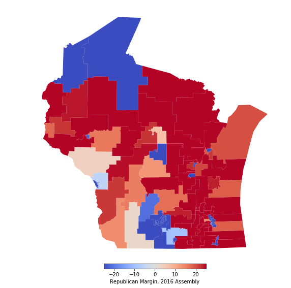
And here’s the turnout by district:
fig, ax = plt.subplots(figsize=(12,11))
ax.axis('off')
plot_df.plot(ax=ax, column='turnout', k=3, linewidth=0.1, cmap='OrRd', legend=True,
    legend_kwds={'label': "Voter Turnout, 2016 Assembly", 'orientation': 'horizontal',
    'pad':0.01, 'shrink':0.3})
plt.show()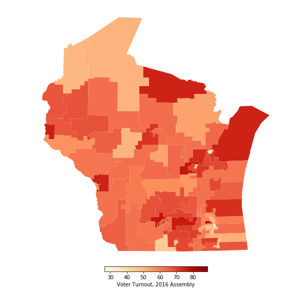
How do these numbers compare to the actual outcomes? Well, I can’t find district turnout results because nobody has the voting age population (VAP) data, but I can look at the cumulative results to get an idea. According to the assembly results, 2,587,171 people voted out of a VAP of 4,461,068, giving a turnout rate of 57.9%. If I sum up my data, I get a vote total of 2,568,160 people out of a VAP of 4,155,055, giving a turnout of 61.8%.
So my approach overstates turnout a little bit because it underestimates the VAP. This makes sense because the synthetic population was created using 2007-2011 Census data and doesn’t take into account population growth since then. But overall I’m pretty happy with these results!
Conclusion
The purpose of this post was to provide a small tutorial on loading and querying synthetic population data in Postgres. I’ve only scratched the surface of what is possible with this data, so stay tuned for future posts on this topic. I think it would be interesting to calculate turnout for every state legislative seat in my dataset, but I would need to move beyond my computer into the cloud to do so. Perhaps I could use something like BigQuery instead.
I really wish the Census Bureau would move towards releasing data in this format. One of the problems with election reporting is that margins often get much more attention than the turnout. This is partly because turnout is very difficult/impossible to calculate for many seats, so having annual synthetic population data available could go a long way towards fixing this problem. This would be especially helpful because, although it’s still useful for other purposes, the synthetic population I used in this post will soon be obsolete for political analysis due to changes in population.
References
[1] Iterative Proportional Fitting. Wikipedia. https://en.wikipedia.org/wiki/Iterative_proportional_fitting
[2] TIGER/Line Geodatabases. US Census Bureau. https://www.census.gov/geographies/mapping-files/time-series/geo/tiger-geodatabase-file.html
[3] A Framework for Reconstructing Epidemiological Dynamics Page. Pitt Public Health Dynamics Lab. https://fred.publichealth.pitt.edu/syn_pops
[4] RTI U.S. Synthetic Household Population. RTI International. https://www.rti.org/impact/rti-us-synthetic-household-population%E2%84%A2
[5] Models of Infectious Disease Agent Study (MIDAS). National Institute of General Medical Sciences. https://www.nigms.nih.gov/Research/specificareas/MIDAS/
[6] Where do voters have the most political influence? Me. https://pstblog.com/2019/03/05/voting-power-comprehensive
[7] 2016 Wisconsin State Assembly Elections. Wikipedia. https://en.wikipedia.org/wiki/2016_Wisconsin_State_Assembly_election#District
[8] Querying PostgreSQL / PostGIS Databases in Python. Andrew Gaidus. http://andrewgaidus.com/Build_Query_Spatial_Database/